Theta*: A Simple Any-Angle Algorithm based on A*
Introduction
Taking a look at ROS1's navigation stack, the global planner's default implementation is either A* or Dijkstra, both of which are classic path planning algorithms that work for navigating simple and structured environments. However, both algorithms fall short when it comes to achieving the true shortest possible path between 2 points. This is where Theta* shines as an any-angle path planner. Theta* is an algorithm built upon A* that relies on line-of-sight to reduce the distance path optimality.
In this brief foray into any-angle path planning, our focus will be on more intuitive visualizations and the comparison of their performance when implemented in the ROS navigation stack. This allows us to make judgements about their strengths and weaknesses in various scenarios. We shall leave aside the more complex sister algorithm, Angle Propagation Theta*, as its time complexity is only marginally better than Theta* yet the paths are less optimal. Here, the graph search problem is represented as a 2D grid map, or a 2D cost map as in the ROS navigation stack.
Why not A*?
The A* planner search is guided by the f-cost heuristic. The f-cost of a cell S is a combination of its g-cost and h-cost:
- g-cost: the shortest distance found thus far from the start cell to S
- _h-cost: A_n estimate of the distance from S to the goal cell.
By means of a sorted open list, the planner will always traverse a cell that minimises the f-cost, and update the costs of existing traversed cells should it find a shorter path in the process.
computeShortestPath(s_start, s_goal):
    g_cost[s_start] = 0
    parent[s_start] = s_start
    openlist = []
    openlist.insert(s_start, g_cost[s_start] + h_cost[s_start])
    closedlist = []
    while openlist NOT empty:
        s = openlist.pop()
        if s == s_goal:
            return “path found”
        closedlist.push(s)
        for s' IN neighbor(s):
            if s' NOT IN closedlist:
                if s' NOT IN openlist:
                    g_cost[s'] = infinity
                    parent[s'] = NULL
                    updateVertex(s, s')
    return “no path found”

updateVertex(s, s'):
    if ( g_cost[s] + cost(s, s') < g_cost[s'] ):
        g_cost[s'] = g_cost[s] + cost(s, s')
        parent[s'] = s
        if s' IN openlist:
            openlist.remove(s')
        openlist.insert(s', g_cost[s'] + h_cost[s'])
Algorithm 1: The classic A*
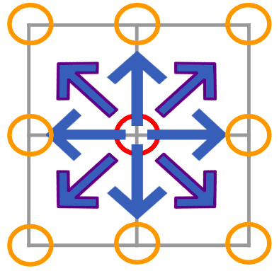
However, as a grid-based planner, A* faces a serious limitation by restricting its search to discrete headings of 45 degrees.

Figure 1: The 8-way connected search direction of A*. Red points is the current vertex and orange points are vertices to be expanded
The true shortest path usually does not adhere to grid lines and can travel along arbitrary headings. This can lead to suboptimal paths for grid based planners like A* as the planner cannot form paths with arbitrary angles.

Figure 2: Grid path versus true shortest path [1]
We can observe these effects by implementing the classic A* algorithm in ROS, where the paths tend to be jagged, constrained to discrete headings of 45 degrees, resulting in paths that are much longer than necessary. The jagged paths are the result of the A* planner following the geometric constraints of the obstacles in the cost map. Figure 3 shows the green path formed by A* to be suboptimal and probably not feasible without an appropriate local planner. This is in comparison to the yellow path which is much closer to the true shortest path. Note: The paths have taken into account the inflation radius of the obstacles.

Figure 3: Blue path is formed by A* and the yellow path is a possible true shortest path
In order to optimize the length of the path, we can add a post processing step to A* that does not require the original algorithm to be modified. This is known as the A* Post-smoothing algorithm [2], which checks for a valid line-of-sight (refer to Appendix A) between the vertices in the existing planned path. Therefore reducing the amount of unnecessary heading changes and also bringing the path closer to an optimal solution.
// For path of length n
AStarPostSmoothing(path):
    k = 0
    t = []
    t.push_back(path[0])
    for i IN range(1,n-1)
        if !lineOfSight(t[k], path[i+1])
            k++
            t.push_back(path[i])
    k++
    t.push_back(path[n])
    return t
Algorithm 2: A* Post-Smoothing
We can observe in Figure 4 that although the green path formed by A* Post-smoothing still has some unnecessary heading changes and waypoints, it is more optimal than the original A* path in Figure 3.

Figure 4: Green path formed by A* Post-Smoothing
The post-smoothing for A* can reduce path lengths to a certain extent, limited by A*'s inability to consider paths that could potentially be shorter. This is illustrated in Figure 5 where A*'s discrete search direction does not allow it to change the side of an obstacle that it travels. Post-smoothing merely checks for the line-of-sight between existing points in the path.

Figure 5: A* Post-Smoothing versus true shortest path [1]
Theta*
To deal with the problem of being unable to consider paths other than those along grid lines or at discrete headings, we cannot separate the planning and post processing step. According to Alex et al. [3]:
A* PS is not guaranteed to find true shortest paths because it only considers grid paths during the A* search and thus cannot make informed decisions regarding other paths during the A* search, which motivates interleaving searching and smoothing.
In fact, Theta* is similar to A* PS except that it interleaves searching and smoothing.
Let's bring our attention to Figure 6. Here, the planner is expanding vertex B3. B3's parent is A4 (the start vertex). And now, the planner is updating the g-cost and parent of the unexpanded cell C3.
In this scenario, Theta* is able to consider both paths 1 and 2, whereas A* will only consider path 1. This is because Theta* checks for line-of-sight between the vertices and their parents during the expansion phase, whereas A* Post-Smoothing only checks for line-of-sight after it has already formed a path.

Figure 6: Scenario 1 of paths 1 and 2 considered by Theta*
By incorporating line-of-sight checks in the updateVertex step from Algorithm 1, we are able to "interleave searching and smoothing". Algorithm 3 shows the steps that lead to the formation of paths 1 and 2. Path 1 is the original A* algorithm whereas path 2 shows the characteristics of the Theta* planner.
updateVertex(s,s')
    if lineOfSight(parent[s], s'):
        /* PATH 2 */
        if g_cost[parent[s]] + cost(parent[s], s') < g_cost(s'):
            g_cost[s'] = g_cost[parent[s]] + cost(parent(s),s')
            parent[s'] = parent[s]
            if s' IN openlist:
                openlist.remove(s')
            openlist.insert(s', g_cost[s'] + h_cost[s'])
    else:
        /* PATH 1 */
        if g_cost[s] + cost(s, s') < g_cost[s']:
            g_cost[s'] = g_cost[s] + cost(s,s')
            parent[s'] = s
            if (s' in openlist):
                open.remove(s')
            openlist.insert(s', g_cost[s'] + h_cost[s'])
Algorithm 3: Basic Theta*
Focusing on path 2, we consider Vertex S and its neighbouring Vertex S'.
IF there is a line-of-sight from the parent of Vertex S to its neighbor Vertex S' then we compare costs to determine IF it is shorter to travel directly from the parent of Vertex S to its neighbour Vertex S', ELSE it does not expand s' and goes on to explore other neighbors of s.
IF there is NO line-of-sight from the parent of Vertex S to its neighbor Vertex S', then the classic A* algorithm will be used for cell expansion.
Taking another example from Figure 7. There is no line-of-sight from the parent of Vertex S (which is S_start) towards S'. Therefore, Theta* will not consider path 1,deeming path 2 the shortest possible path towards the goal.

Figure 7: Scenario 2 of paths 1 and 2 considered by Theta*
An implementation of Theta* in ROS (Figure 8) shows that there are lesser unnecessary heading changes and that the path obtained is much closer to the true shortest path.

Figure 8: Theta* planner in ROS
But of course, looks are often deceiving and we need to compare the path lengths from the algorithms we have discussed earlier. Testing the planners on 3 different paths gives us the following results, which is mildly surprising as it indicates that even as Theta* theoretically yields shorter paths than A* Post-smoothed, it is only marginally shorter. The choice between A* Post-Smoothed and Theta* will depend on how much computational resources one is willing to trade for a shorter path. It is possible that in a very large cost map, there are more benefits to be reaped as the optimization makes more of a difference in path lengths.
Path A
 A*: 22.25 m
 A* Post-smoothed: 21.76 m
 Theta*: 21.53 m
Path B
 A*: 22.36 m
 A* Post-smoothed: 22.14 m
 Theta*: 21.75 m
Path C
 A*: 22.25
 A* Post-smoothed: 21.76
 Theta*: 21.53
Figure 9: Comparison table of path lengths for A*, A*PS and Theta*
Conclusion
It has been shown through the ROS navigation stack that Theta* does indeed optimize the path length and reduce unnecessary heading changes, albeit only marginally compared with A* Post-Smoother. The benefits of using Theta* will depend on the size of the environment and the situation. One situation where the more computationally expensive Theta* could pay off, would be in large cluttered cost maps where the optimization could result in robots travelling a lot less distance as compared with using A* or its post-smoothed version.
On the other hand, there are also numerous problems associated with Theta* that have not been considered. An inherent limitation is obstacle-hugging which can lead to collision with obstacles without an inflation radius. Even so, increasing the inflation radius could lead to narrow walkways becoming untraversable. Another major problem is that Theta* ignores the kinematic constraints of the robot and plans paths that are piecewise linear with no continuity, requiring the paths to undergo further post processing to yield a kinematically feasible path.
The problems faced by Theta* are also recurring issues in the vast world of path planners. Other types of planners have sought to overcome these limitations and found success in various domains. The more notable ones are Hybrid A* [4] and State Lattice Planner [5], which are deterministic algorithms that have proved their effectiveness at the DARPA Grand Challenge. These planners will be the focus of a future discussion with a detailed study at their performance within the ROS framework.
Appendix A
ROS: The planners were implemented on the ROS kinetic stack and tested on turtlebot3_house world in Gazebo.
Line-of-sight algorithm:
LineOfSight(s, s'):

    x0 = s.x
    y0 = s.y;
    x1 = s'.x
    y1 = s'.y;

    dy = y1-y0
    dx = x1-x0;

    f = 0

    if (dy < 0):
        dy = -dy
        s.y = -1
    else:
        s.y = 1

    if dx < 0:
        dx = -dx
        s.x = -1
    else:
        s.x = 1

    if (dx >= dy):
        while (x0 != x1):
            f = f + dy
            if (f >= dx ):
                if grid(x0+((s.x-1)/2), y0 + ((s.y-1)/2)):
                    return false
                y0 = y0 + s.y
                f = f - dx
            if f != 0 AND grid(x0+((s.x-1)/2), y0 + ((s.y-1)/2)):
                return false
            if dy = 0 AND grid(x0 + ((s.x-1)/2), y0) AND grid(x0 + ((s.x-1),2), y0-1):
                return false
            x0 = x0 + s.x

    else:
        while (y0 != y1):
            f = f + dx
            if (f >= dy)
                if grid(x0 + ((s.x - 1)/2), y0 + ((s.y-1)/2)) :
                    return false;
                x0 = x0 + s.x
                f = f - dy
            if f!=0 AND grid(x0+((s.x-1)/2), y0 + ((s.y-1)/2)):
                return false;
            if dx=0 AND grid(x0, y0+((s.y-1)/2)) AND grid(x0-1 , y0 + ((s.y-1)/2)):
                return false
            y0 = y0 + s.y

    return true
Algorithm 4: Line-of-Sight
References
[1] K. Daniel, A. Nash, S. Koenig, and A. Felner, “Theta*: Any-Angle Path Planning on Grids,” Journal of Artificial Intelligence Research, vol. 39, pp. 533–579, 2010.
[2] C. Thorpe and L. Matthies, “Path Relaxation: Path Planning for a Mobile Robot,” Oceans 1984, 1984.
[3] A. Nash and S. Koenig, “Any-Angle Path Planning,” AI Magazine, vol. 34, no. 4, p. 85, 2013.
[4] Dmitri Dolgov, Sebastian Thrun, Michael Montemerlo, and James Diebel. Practical search techniques in path planning for autonomous driving. 2008.
[5] T. M. Howard, C. J. Green, A. Kelly, and D. Ferguson, “State space sampling of feasible motions for high-performance mobile robot navigation in complex environments,” Journal of Field Robotics, vol. 25, no. 6-7, pp. 325–345, 2008.