Introduction

Many mobile robot path plannings are done in grid maps, especially if it is a ground robot operating in a planar environment. Indeed, widely-used ROS packages are available to support this way of operation, such as gmapping and navfn.

However, we sometimes wish to to add semantic information to our grid map, such as, only the left side of this corridor may be used, or this door is not for robots, or keep left on this hallway. To enhance our grid map with these, we propose to use graphs.

A graph is a mathematical structure where we have vertices connected with edges. The vertices may contain values and the edges may be directed and weighted.

In our graph map, the vertices represent coordinates in the gird map, the edges are directed and their weights are the euclidean distances between the two vertices they connect.

There are two main advantages of enhancing a grid map with a graph map:

1. Graph map is "smaller" than grid map

Think of the grid map as a graph map where each grid cell is a vertex connected to its 8 neighbours with bidirectional edges. When running a planning algorithm, such as A*, these cells are going to be expanded one at a time, each adding up to another 8 to the queue. These algorithms are fast, but larger maps would still mean a lot of computation.

A carefully designed graph map would have much fewer vertices; just a handful per room. This would reduce the complexity of planning in graph maps.

2. Graph map can have semantically meaningful edges

Only vertices that may be directly reached from each other are connected by an edge. This can of course mean that two points in space that are not obstructed are connected with an edge, but it can also mean that the robot may only move between predefined points regardless of surrounding free space.

For instance, imaging setting vertices along the left side of a wide corridor. This will restrict planning to that side of the corridor, effectively creating a lane. If we make this lane one way by making the edges directional, and create another one-way lane in the opposite direction on the other side of the corridor, and only connect the two lanes at the far ends of the corridor, we can control the flow of robot traffic.

Further, since weights can be assigned to edges, we can also bias the planning to behave one way than another. Imagine dynamically assigning weights to discourage robots from planning through busy areas such as another robot’s working area or places with a lot of human foot traffic.

Illustrated Example

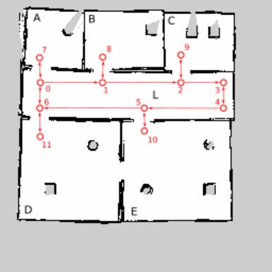
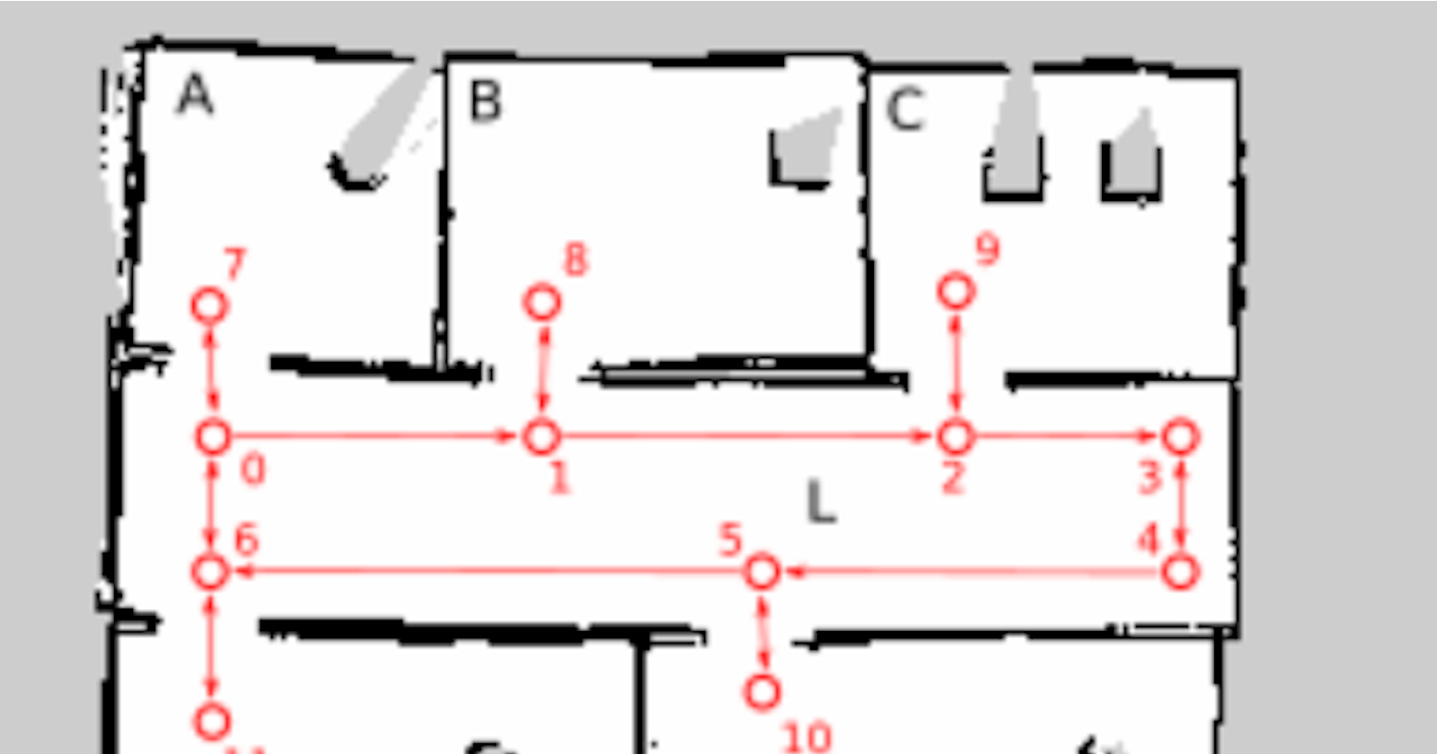
Figure 1. Graph map (red) overlaid on grid map. Vertices are numbered 0 through 11, rooms are labelled with letters A through E, and L. Double-sided arrows are bidirectional edges, single-sided ones are directed

Consider Figure 1. We have a building with five rooms labelled A through E and a corridor connecting them, labelled L. Rooms D and E are connected with a door.

With planning on a grid map, we can plan a robot navigation between any free points in the map, usually on a shortest distance criterion. The size of such a (global) plan is at least the number of pixels between the starting point and the goal.

With a graph map, we can add constraints to the planner. For example, the corridor is divided into two lanes (vertices 1, 2, 3, 4 for left to right movement, and vertices 5, 6, 7 for right to left movement), and changing sides is only possible at the leftmost and rightmost ends of the corridor. If we make the (1, 7) and (4, 5) edges directed, then the corridor functions like a roundabout.

In the graph map, movement from room D to room E must go through the corridor, as there is no (11, 12) edge. Effectively, we are forbidding the robot from using the doorway between the two rooms.

Also, the graph map has 12 vertices and 12 edges, while the grid map has a 256 x 256 px resolution.

Graph Representation

Graph type. We will use directed graphs so that we can define one-way lanes. When a lane is two-way, we can simply use two edges. This also means we can differentially weight the two directions.

Vertex. Since this graph map represents a physical space, its vertices must contain information of its real-space coordinate in (x, y, z) or (x, y).

Edge. Edges are directed and have weights. In scenarios where weights are not important, we can just set them to one. In addition to weights, edges in our graph shall also have a length property, set to the euclidean distance between the vertices at their ends. We can use the length as the distance property when doing shortest path search, or we can multiply length with weight to prioritise some edges over another.

Just like the grid map, it must be possible to save the graph map to file and load them at a later time. However, while grid map is the output of a mapping run, the graph map would be the output of a translation from the grid map, and so it must be made after the grid map.

The translation step from grid map to graph map can be as simple as a human specifying vertices and edges in a spreadsheet, a utility to graphically define graph on a grid map, to an automated method. We have prototyped the manual method.

Off-Graph Planning

The pose of our robots would not be always coincident with the graph vertices. Similarly with the goal point. In fact, since the graph vertices represent points, these robot points would practically never be coincident with the graph vertices. To perform complete planning, we then need to make accommodation to these off-graph points.

We add the start and goal points into the graph to perform graph planning to and from arbitrary poses. Those points can be trivially made into vertices, but deciding what edge should connect them to the rest of the graph needs more consideration.

Our approach to off-graph planning has two components: the two-vertex rule and the line-of-sight check.

Two-Vertex Rule

When creating edges from off-graph points to graph vertices, we connect them to their two closest neighbour. This is the two-vertex rule. The reasoning is explained in below.

Suppose we have a simple graph with three vertices as shown below (green), and our start and goal are the red and blue vertices respectively.

Suppose we connect the new start and goal vertices to the closest vertex already in the graph (by euclidean distance). We can then plan with this new graph.

However, when our start and goal vertices are not neatly aligned with in-graph vertices, we may get a result like below:

This plan makes the robot “backtrack” to vertex 0, follow the graph to vertex 2, then “backtrack” again to the goal. We can improve upon this scheme by connecting the start and goal vertices to two closest vertices already in the graph, like so:

When we perform shortest path search in this resulting graph, the robot will go from start to vertex 1 then to goal, like shown below (red arrows).

In more practical scenarios, there would be several vertices between start and goal instead of just one in this example.

Line-of-Sight Check

The graph does not know about walls. Connecting two close vertices might mean drawing a path through a wall. The local planner might not let the robot to hit the wall, but it nevertheless get a less than efficient route to its destination.

To solve this, we let the graph planner access the grid map (so now the grid map has a graph map and it has a grid map). When we apply the two-vertex rule for off-graph planning, we find a plan in grid map between the new vertex to the pair of closest vertex. Since grid map does know about walls, we can inspect the returned plan to check if any of the closest vertex has obstacle-free line-of-sight. The criterion we use is if the returned plan is shorter than a multiplier (1.5x) of the euclidean distance between the new vertex to the closest in-graph vertex, then there is line-of-sight, and we add an edge between the vertices. If there are no nearest neighbours with line-of-sight, we expand the search to four nearest neighbour. We keep doubling the number of neighbours to be considered until we get one with line-of-sight or we have covered the entire graph (report failure).

Doing grid search in addition to the graph search may seem to negate one of the advantages of having a graph map in the first place, but it is not necessarily the case. Since we are doing grid search only for closest vertices, the search space is limited. And in larger maps, we can load only the part of the grid map immediately relevant to the line-of-sight evaluation.

Vertex Placement Consideration

From our experiments, there are a few best practices for placing vertices in the graph map for good results:

• Place vertices in a thoroughfare (that is, not room) outlining the path you would like the robot to take when traversing the region
• Space vertices such that there are several within the range of your local planner so that it will plan to vertices instead of to the limit of its local map
• Place a vertex in a room near the entrance. Use this vertex or somewhere close to plan navigation into the room
• Place vertices around the perimeter of a room such that the closest vertex to a robot in arbitrary pose inside the room is one of said perimeter vertices
• Connect above perimeter vertices to the entrance vertex directly, unless you would like to define set paths within the room. This is to facilitate planning out of a room when the robot finishes doing its task away from the entrance, and to prevent planning using vertices from the adjacent room; the graph does not know about walls.

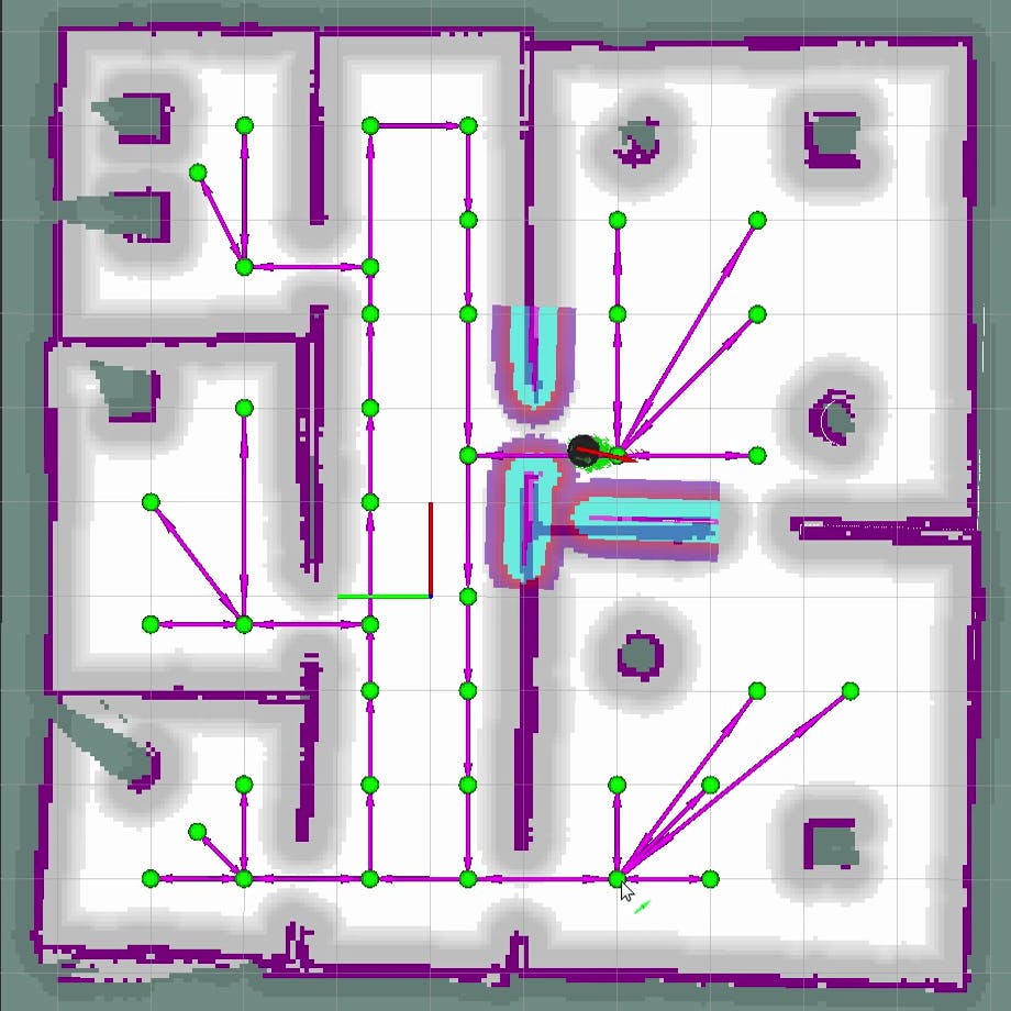
Figure 2. Example detailed graph overlaid on graph map. The middle corridor has two one-way lanes, each room has entrance vertices and perimeter vertices

Integration with Planners

Replanning and Path Truncation

A path planner may be periodically called with the same goal to account for changes in the environment. Graph maps do not change, and periodically querying it for path may even result in inconsistent path, as the position of the robot at each replan will be added to the graph with the two-vertex rule, and depending on its deviation from the graph path (e.g. while avoiding obstacle with the local planner), the plan may "jump lanes". For this reason, instead of redoing the graph search when asked to replan, our graph planner instead truncate the existing plan to the section between current robot position and goal.

At each replan request, we compare the start (current robot position) with the plan from previous cycle (which is a sequence of poses from start to goal). For every pose in the plan in order, if the start is ahead of it, then the pose is skipped, if start is behind it then, then we return the path from there, prepending the start.

To evaluate the aheadness of the start point p_i to a vertex v_j, we take the dot product of the vector a = (p_i - v_j) and b = (v_j+1 - v_j). If it is negative, then the point is behind the vertex. Otherwise the point is ahead of v_j. We then divide the dot product with the magnitude of b vector (effectively taking the ratio between projection of a to b and magnitude of b), if it is larger than one, then the point is ahead of v_j+1 too. This aheadness evaluation is illustrated below.

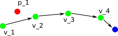
Replanning with path truncation. Existing path is represented by the green vertices, robot current pose is p_1 and goal (unchanged from previous cycle) is blue.

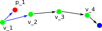
Is p_1 ahead or behind v_1? We test with the two blue arrows. The dot product is positive, so p_1 is ahead of v_1. But the projection of the (p_1 - v_1) vector is shorter than the magnitude of the (v_2 - v_1) vector, so p_1 is behind v_2.

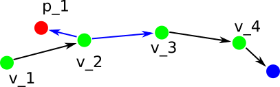
p_1 is behind v_2 because the dot product of the two vectors denoted by the blue arrows is negative

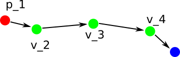
Resulting path on replan, v_1 is removed and p_1 is prepended, but the rest remain the same

Global Planner on Graph, Local Planner on Grid

A graph map would not have explicit obstacles. Its vertices must of course be specified in free spaces in the static map, but an edge does not necessarily mean a straight, obstacle-free path between the connected vertices (although it can be made to be so). By itself, it is not suitable for local planning. Also, dynamic obstacles or small changes in the environment are invisible to the graph map.

When combined with a local planner, we can have a lighter weight global planner (in graph!) while maintaining the safety/smoothness/etc desiderata with the local planner.

The graph map does not have anything to do with localisation. AMCL, for instance, would still use the static grid map.

Different Modes of Global Planning

There are scenarios where we still want to perform global planning on a grid map, e.g. the case where a robot is tasked to follow a trajectory that “paints” a room (e.g. cover the entire floor space for cleaning). With global planning on a grid map, the global plan specifies the high-level cleaning path, while the local planner plans the detailed route between points in the global path. If we replace the global planner with a graph-based planner using a graph map, we have to à priori include the coverage path as part of the graph. If we do not, and put the room as a single node in the graph, then the coverage path must be done in the local planner, and that precludes covering a room larger than the window of the local planner.

A solution to this is to have two modes of global planner: graph-planner for long-range movement in the map, and grid-planner for in-room planning.

Figure 3. Scenario where two modes of global planning are necessary. Graph-based (red) between rooms and grid-based (green) for coverage planning within a room

One such scenario needing two modes of global planning is illustrated in Figure 3. For movement between rooms, we can use a graph-based planner to coordinate multiple robots, save computation time, and respect corridor lanes. Within a room, we switch to a grid-based planner with task-specific criteria, such as cleaning coverage. When the robot has completed its in-room task, it can switch back to graph-based planner to move on to the next room.

In our prototype we wrap both the grid and graph planner in a general planner package and switch the active planner as needed.

Conclusion

In this article we have presented the advantages of a graph map: smaller search space and semantically meaningful edges.

We have also presented planning to and from off-graph points with the two-vertex rule and line-of-sight check.

Finally, we have described ideas for replanning with path truncation and integrating multiple methods of global planning.